Note

This is a Quarto document which nicely combines both R code, its results and text explanation to enable an easy and interactive access for both learners, readers and supervisors to such analyses. To learn more about Quarto see https://quarto.org. By default all code lines are blended, but you can show them by clicking on the code button.

1 Introduction

Tip

For more information about Seurat R package please visit a dedicated documentation page with all details regarding embedded functions and their usage. If you use custom packages in your publications, do not forget to cite them using the information provided at the maintainers web-site.

Seurat is a common R package for comprehensive scRNA-seq analysis

This is a basic Seurat analysis of scRNA-seq data downstream of CellRanger pipeline. The reference paper authors previously assembled feature count matrix, metadata and row data Seurat object and uploaded it on GEO repository. Analysis in this document is required before annotating specific cell types and analyzing differential gene expression. We aim to have dimensionality reduction data like tSNE or UMAP available for visualizing results further. This analysis was taken from a youtube tutorial almost without modifications, but using current dataset.

2 Loading data and dependencies

For this analysis we need Seurat and tidyverse packages

Code

library(Seurat)
library(tidyverse)

Loading our dataset

Code

data.initial <- readRDS("./../input/GSE238137_blood-liver_MAIT-Tmem_seurat.rds")
data.initial

An object of class Seurat 
39947 features across 89456 samples within 5 assays 
Active assay: SCT (17646 features, 0 variable features)
 3 layers present: counts, data, scale.data
 4 other assays present: RNA, ADT, HTO, integrated
 2 dimensional reductions calculated: pca, umap

3 Running standard Seurat analysis

3.1 Dataset reduction

Let’s reduce our seurat object until desired cell populations and assays

3.1.1 Remove all assays except RNA seq

Code

DefaultAssay(data.initial) <- "RNA" # to allow other assay layers to be deleted

data.initial <-  DietSeurat(
  data.initial,
  features = NULL,
  assays = "RNA",
  dimreducs = NULL,
  graphs = NULL,
  misc = TRUE)

3.1.2 Let’s select only Experiment 2 and liver tissue samples

Code

data.mait.Tmem.2exp <- data.initial[, data.initial$experiment == "Exp 2"] 

data.liver.mait.Tmem.2exp <- data.mait.Tmem.2exp[, data.mait.Tmem.2exp$tissue == "Liver"] 
data.liver.mait.Tmem.2exp

An object of class Seurat 
19289 features across 17069 samples within 1 assay 
Active assay: RNA (19289 features, 0 variable features)
 2 layers present: counts, data

3.2 Quality control

3.2.1 Filtering low-quality cells based on % of mitochondrial gene transcripts

Let’s first calculate the percentage of mitochondrial gene transcripts using build-in Seurat function

Code

data.liver.mait.Tmem.2exp[["percent.mt"]] <- PercentageFeatureSet(data.liver.mait.Tmem.2exp, pattern = "^MT-")
Idents(data.liver.mait.Tmem.2exp) <- data.liver.mait.Tmem.2exp$cell_type

Plotting Violin plot showing all information about QC metrics

Code

VlnPlot(data.liver.mait.Tmem.2exp, features = c("nFeature_RNA", "nCount_RNA", "percent.mt"), ncol = 3)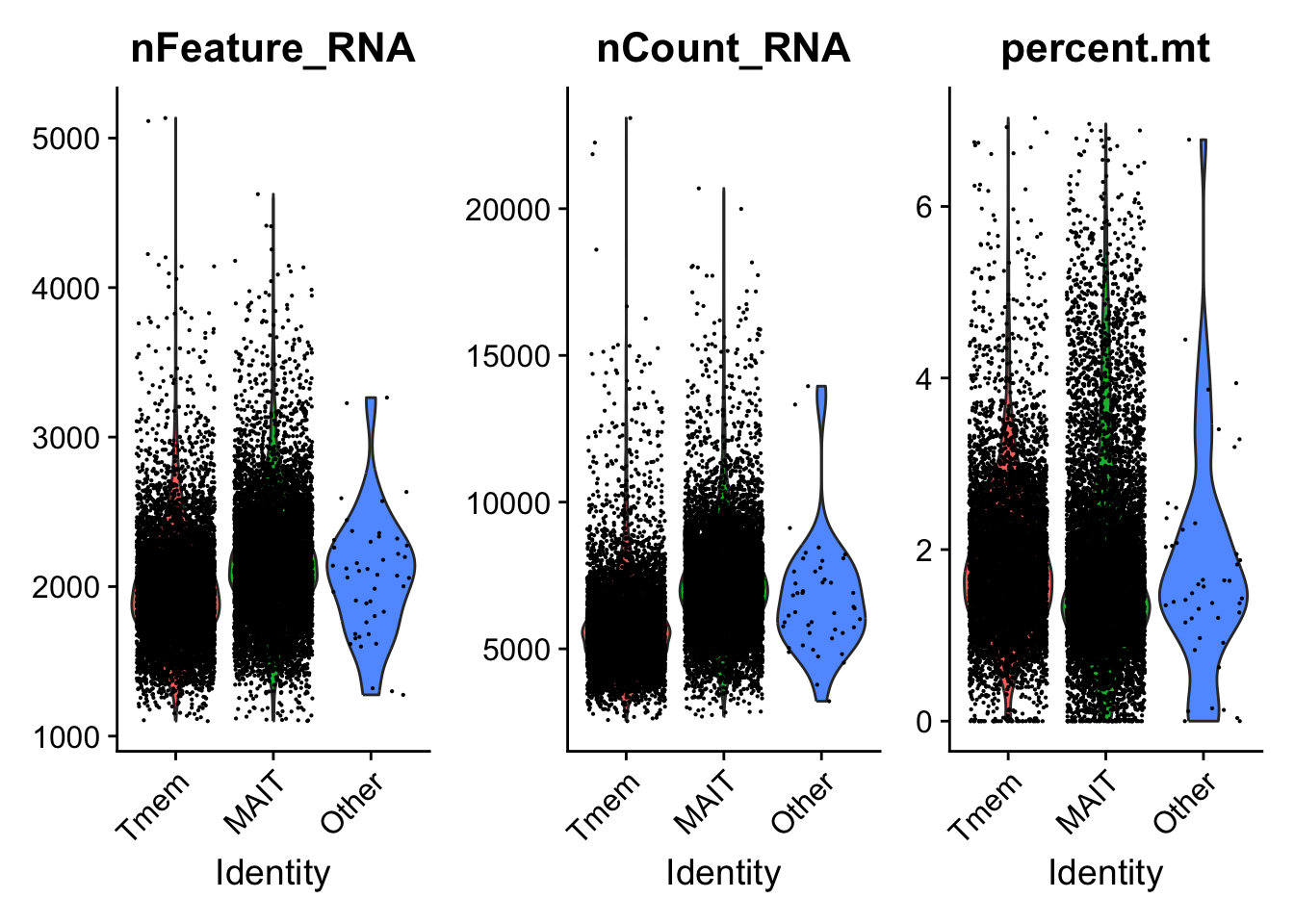

We can see that the overall amount of cells with mito DNA % > 5 is very small indicating high quality of cell transcriptomes contained in the dataset. One of the main reasons to exclude cells with an unusually high number of detected genes is the suspicion that such cells might actually be doublets or multiplets. Doublets occur when two cells are mistakenly captured as a single cell during the cell isolation process. This results in a higher total gene count than typically observed in single cells because the transcriptomes of two (or more) cells are combined

And FeatureScatter plot

Code

FeatureScatter(data.liver.mait.Tmem.2exp, feature1 = "nCount_RNA", feature2 = "nFeature_RNA") +
  geom_smooth(method = 'lm')

`geom_smooth()` using formula = 'y ~ x'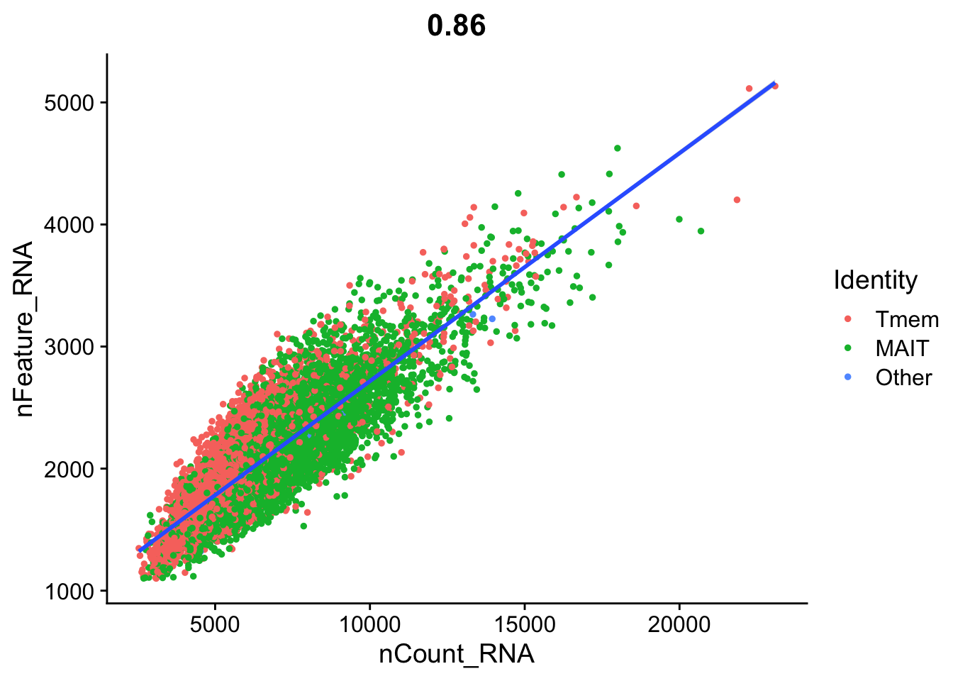

This plot ensures that there are little cells with uncorrelated transcripts rate identification and the total number of RNA counts

In our case the authors already performed QC filtering, so we skip this step.

Code

# data.liver.mait.Tmem.2exp <- subset(Garner.Trem.2exp, subset = nFeature_RNA > 200 & nFeature_RNA < 2500 & percent.mt < 5)

3.3 Proceeding with standard downstream analysis steps to identify cell clusters and plot UMAP

3.3.1 Normalize data and find variably expressed genes

Code

data.liver.mait.Tmem.2exp[["RNA"]]@meta.features <- data.frame(row.names = rownames(data.liver.mait.Tmem.2exp[["RNA"]])) # Assign to Seurat objects rownames correctly
data <- NormalizeData(data.liver.mait.Tmem.2exp) 
data <- FindVariableFeatures(data)

3.3.2 Identify the 10 most highly variable genes

Code

top10 <- head(VariableFeatures(data), 10) 
top10

 [1] "HSPA6"  "HSPA1A" "CCL20"  "HSPA1B" "CCL4L2" "GNLY"   "CCL3L1" "CCL3"  
 [9] "EGR1"   "XCL1"

3.3.3 Scaling

Code

all.genes <- rownames(data)
data <- ScaleData(data, features = all.genes)

Centering and scaling data matrix

3.3.4 Perform Linear dimensionality reduction

3.3.5 Visualize PCA results

Code

print(data[["pca"]], dims = 1:5, nfeatures = 5)

PC_ 1 
Positive:  HLA-DRB1, GZMH, XCL2, HLA-DPA1, ARID5B 
Negative:  KLRB1, IL7R, SLC4A10, CEBPD, RORA 
PC_ 2 
Positive:  NR4A2, ACTB, DUSP2, IER2, PPP1R15A 
Negative:  MT-ND3, HLA-G, MT-CYB, FTH1, PDE3B 
PC_ 3 
Positive:  METRNL, PPP2R5C, FAM177A1, TUBB4B, VPS37B 
Negative:  RPS26, TXNIP, MYL12A, ANXA1, CD52 
PC_ 4 
Positive:  DUSP4, COTL1, ZFP36, ATP1B3, ALOX5AP 
Negative:  NKG7, FGFBP2, FCGR3A, GZMB, GNLY 
PC_ 5 
Positive:  JUND, ZFP36, DUSP2, MAFF, PPP1R15A 
Negative:  SAMSN1, ARRDC3, MALAT1, GLIPR1, ITK

Code

DimHeatmap(data, dims = 1, cells = 500, balanced = TRUE)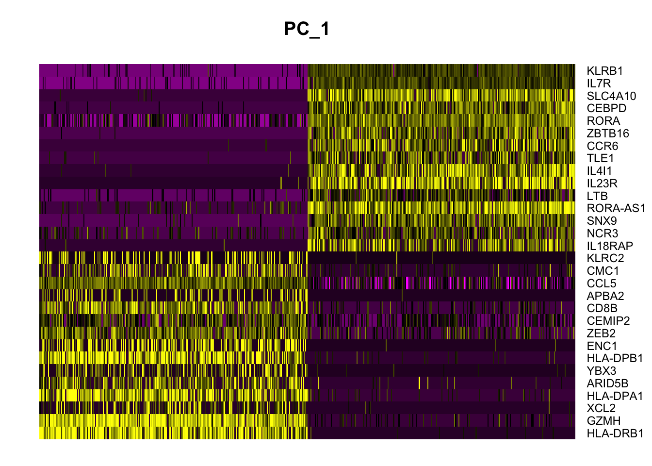

3.3.6 Determine dimensionality of the data

Code

ElbowPlot(data)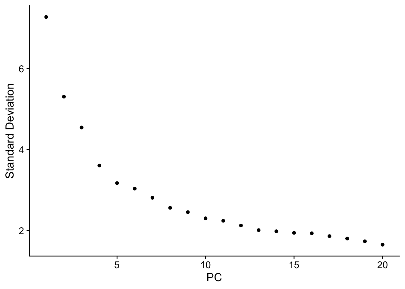

Elbow plot is also sometimes called scree plot. After certain number of PCA captured variation is expected to drop down. Since subsequent PCAs are less informative, this sudden drop resembles elbow shape

3.3.7 Clustering

Visualize PCA plot with clusters

Code

DimPlot(data, reduction = "pca", group.by = "RNA_snn_res.0.5", label = TRUE)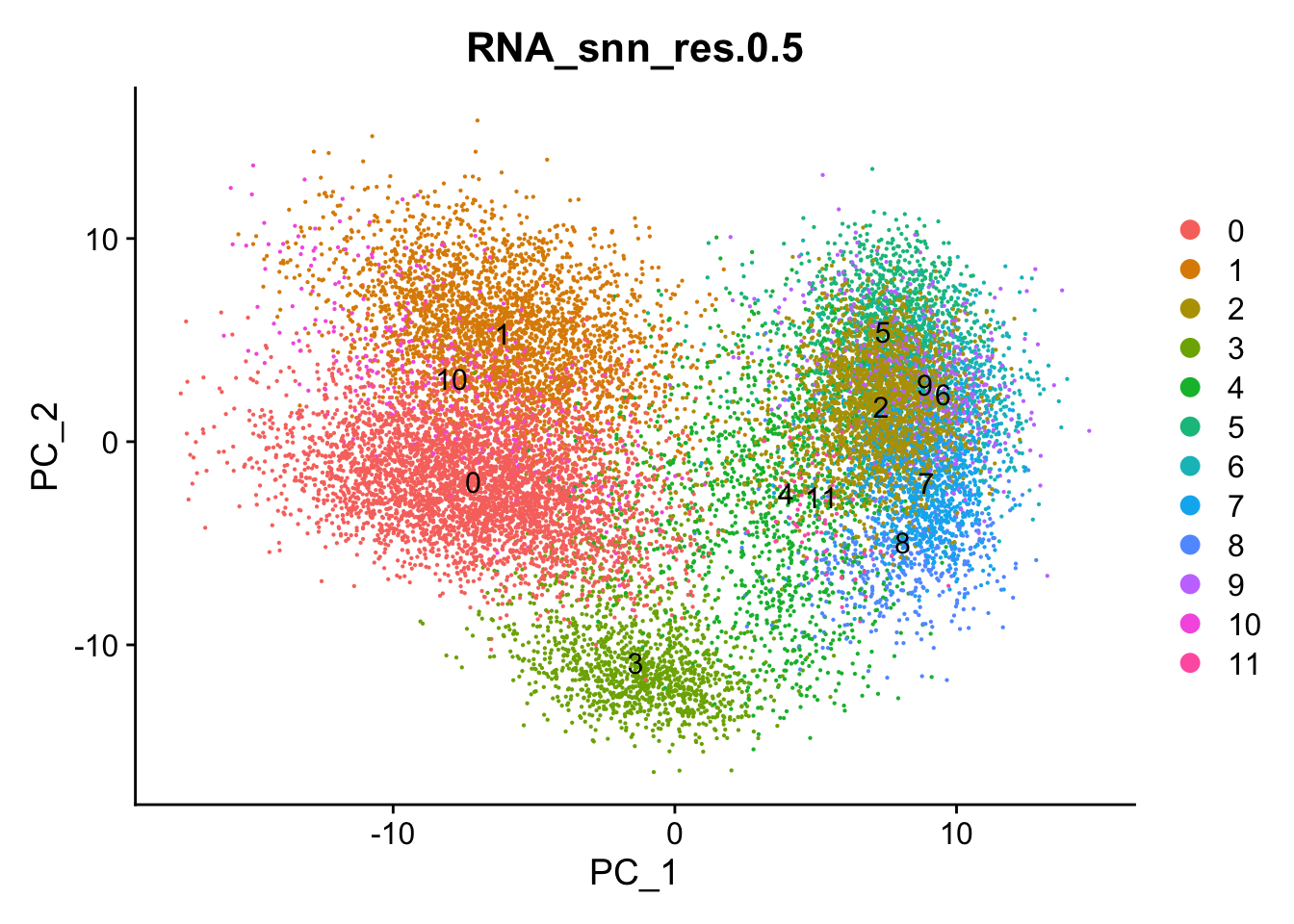

Code

Idents(data) <- "RNA_snn_res.0.5"

3.3.8 Create the UMAP map

Plot UMAP to visualize clusters spatial distribution

Code

DimPlot(data, reduction = "umap", group.by = "RNA_snn_res.0.5")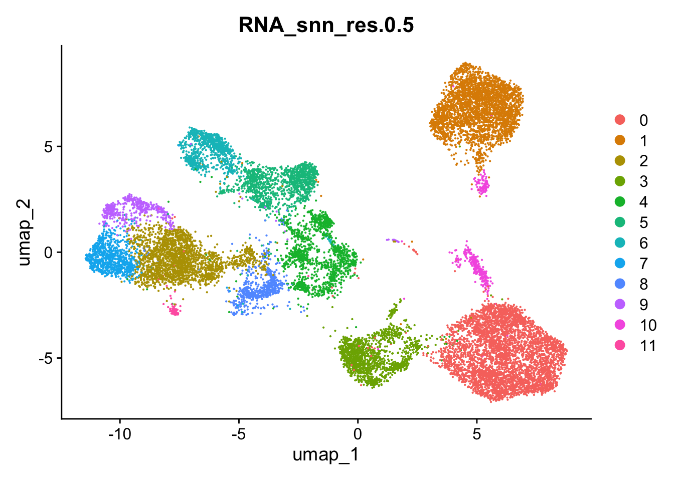

3.3.9 Save our analyzed Seurat object for downstream analyses

Code

data

An object of class Seurat 
19289 features across 17069 samples within 1 assay 
Active assay: RNA (19289 features, 2000 variable features)
 3 layers present: counts, data, scale.data
 2 dimensional reductions calculated: pca, umap

Code

#saveRDS(data, file = "./../output/Garner.seurat.2exp.liver.mait_analyzed.rds")

Code

sessionInfo()

R version 4.3.3 (2024-02-29)
Platform: aarch64-apple-darwin20 (64-bit)
Running under: macOS Sonoma 14.3

Matrix products: default
BLAS:   /Library/Frameworks/R.framework/Versions/4.3-arm64/Resources/lib/libRblas.0.dylib 
LAPACK: /Library/Frameworks/R.framework/Versions/4.3-arm64/Resources/lib/libRlapack.dylib;  LAPACK version 3.11.0

locale:
[1] en_US.UTF-8/en_US.UTF-8/en_US.UTF-8/C/en_US.UTF-8/en_US.UTF-8

time zone: Europe/Zurich
tzcode source: internal

attached base packages:
[1] stats     graphics  grDevices utils     datasets  methods   base     

other attached packages:
 [1] lubridate_1.9.3    forcats_1.0.0      stringr_1.5.1      dplyr_1.1.4       
 [5] purrr_1.0.2        readr_2.1.5        tidyr_1.3.1        tibble_3.2.1      
 [9] ggplot2_3.5.0      tidyverse_2.0.0    Seurat_5.0.3       SeuratObject_5.0.1
[13] sp_2.1-3          

loaded via a namespace (and not attached):
  [1] RColorBrewer_1.1-3     rstudioapi_0.16.0      jsonlite_1.8.8        
  [4] magrittr_2.0.3         spatstat.utils_3.0-4   ggbeeswarm_0.7.2      
  [7] farver_2.1.1           rmarkdown_2.26         vctrs_0.6.5           
 [10] ROCR_1.0-11            spatstat.explore_3.2-7 htmltools_0.5.8.1     
 [13] sctransform_0.4.1      parallelly_1.37.1      KernSmooth_2.23-22    
 [16] htmlwidgets_1.6.4      ica_1.0-3              plyr_1.8.9            
 [19] plotly_4.10.4          zoo_1.8-12             igraph_2.0.3          
 [22] mime_0.12              lifecycle_1.0.4        pkgconfig_2.0.3       
 [25] Matrix_1.6-5           R6_2.5.1               fastmap_1.1.1         
 [28] fitdistrplus_1.1-11    future_1.33.2          shiny_1.8.1.1         
 [31] digest_0.6.35          colorspace_2.1-0       patchwork_1.2.0       
 [34] tensor_1.5             RSpectra_0.16-1        irlba_2.3.5.1         
 [37] labeling_0.4.3         progressr_0.14.0       fansi_1.0.6           
 [40] spatstat.sparse_3.0-3  timechange_0.3.0       mgcv_1.9-1            
 [43] httr_1.4.7             polyclip_1.10-6        abind_1.4-5           
 [46] compiler_4.3.3         withr_3.0.0            fastDummies_1.7.3     
 [49] MASS_7.3-60.0.1        tools_4.3.3            vipor_0.4.7           
 [52] lmtest_0.9-40          beeswarm_0.4.0         httpuv_1.6.15         
 [55] future.apply_1.11.2    goftest_1.2-3          glue_1.7.0            
 [58] nlme_3.1-164           promises_1.2.1         grid_4.3.3            
 [61] Rtsne_0.17             cluster_2.1.6          reshape2_1.4.4        
 [64] generics_0.1.3         gtable_0.3.4           spatstat.data_3.0-4   
 [67] tzdb_0.4.0             data.table_1.15.4      hms_1.1.3             
 [70] utf8_1.2.4             spatstat.geom_3.2-9    RcppAnnoy_0.0.22      
 [73] ggrepel_0.9.5          RANN_2.6.1             pillar_1.9.0          
 [76] spam_2.10-0            RcppHNSW_0.6.0         later_1.3.2           
 [79] splines_4.3.3          lattice_0.22-6         survival_3.5-8        
 [82] deldir_2.0-4           tidyselect_1.2.1       miniUI_0.1.1.1        
 [85] pbapply_1.7-2          knitr_1.45             gridExtra_2.3         
 [88] scattermore_1.2        xfun_0.43              matrixStats_1.2.0     
 [91] stringi_1.8.3          lazyeval_0.2.2         yaml_2.3.8            
 [94] evaluate_0.23          codetools_0.2-20       cli_3.6.2             
 [97] uwot_0.1.16            xtable_1.8-4           reticulate_1.35.0     
[100] munsell_0.5.1          Rcpp_1.0.12            globals_0.16.3        
[103] spatstat.random_3.2-3  png_0.1-8              ggrastr_1.0.2         
[106] parallel_4.3.3         dotCall64_1.1-1        listenv_0.9.1         
[109] viridisLite_0.4.2      scales_1.3.0           ggridges_0.5.6        
[112] leiden_0.4.3.1         rlang_1.1.3            cowplot_1.1.3